Basics of Medical statistics

Statistics

Statistics is the discipline that concerns the collection, organization, analysis, interpretation and presentation of data

Medical Statistics

Medical statistics deals with applications of statistics to medicine and the health sciences, including epidemiology, public health, forensic medicine, and clinical research. Medical statistics is a subdiscipline of statistics. "It is the science of summarizing, collecting, presenting and interpreting data in medical practice, and using them to estimate the magnitude of associations and test hypotheses. It has a central role in medical investigations. It not only provides a way of organizing information on a wider and more formal basis than relying on the exchange of anecdotes and personal experience, but also takes into account the intrinsic variation inherent in most biological processes."

Two main branches of statistics

Descriptive statistics - The discipline that deals with the description, representation and visulaisation of data. It summaries the findings but it does not generalize a population from a given sample.

Inferential statistics - Other main branch of statistics. Inferential statistics use a random sample of data taken from a population to describe and make inferences about the population. Inferential statistics are valuable when examination of each member of an entire population is not convenient or possible. For example, to measure all the patients (whole population) with a symptom (e.g. hypertension) is usually not possible. You can measure the data on a representative random sample of patients with the symptom. You can use the information from the sample to make generalizations about the whole population of patients with the symptom (e.g. hypertension). Inferential statistics is about hypotheses testing.

Data

There are two main types of data, Both can be further divided into two subgroups:

1. Qualitative Data: It is description of quality of something for example: level, appearance, taste. Can be categorised.

• Ordinal data: Ordinal data is a specific subcategory of qualitative data. It deals with categories that can be organized in some logical sequence known as “rank order”, e.g. level of education (Elementary school, Secondary school, University)

• Nominal data: type of data that is used to label variables. Unlike ordinal data, nominal data cannot be ordered and cannot be measured

2. Quantitative Data: It is information that can be measured and presented as numbers

• Discrete: it can only take certain values. Can only be divided into discrete values i.e. whole numbers. For example; The number of compliments your department receives per week or the weekly number of cardiac arrests represent types of quantitative-discrete data.
• Continuous: Continuous data can take any value (within a range). Everyday examples include SaO2, blood pressure and weight, height, etc.

Summarizing Data

Summarizing data is important because it allows the information to be easily and quickly interpreted. It can be done graphically or in a tabular format- depending upon the type of presentation.

Tabular Summary

These are commonly used to summaries nominal data but they can be applied to ordinal and quantitative varieties as well. The number within a particular category is called the frequency. Consequently, a frequency table lists the various numbers within different categories.

Graphical Summary

histogram

There are several ways of graphical summarizing of information (for example: Scatter plot, Line chart, Bar chart, Pie chart) the choice depends upon the type of data you are dealing with.

• Frequency distribution- is an organized graphical presentation of the number of individuals for each value on the scale of measurement. It allows the researcher to have a look at the entire data. It shows whether the observations are high or low and also their concentrations, i.e. if they are concentrated in one place or they spread out. Thus, frequency distribution presents a picture of how the individual observations are distributed in the measurement scale.
  • Histogram: the most commmon graphical representation of frequency distribution. The data in the histogram are shown as rectangles representing different categories, or bins, there is no overlap between them. ​Each rectangle represents the corresponding absolute or relative frequency when the horizontal axis (X axis) represents the categories of data (bins, intervals) and the vertical axis (y axis) depicts the frequency. Height of the rectangle, expresses the frequency of cases. The bins (intervals) must be adjacent, and are often (but are not required to be) of equal size. The words used to describe the patterns in a histogram are: "symmetric", "skewed left", "skewed right", "unimodal", "bimodal",“multimodal.

Normal distribution

normal distribution

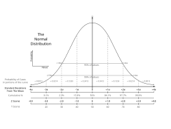
Bell-shaped frequency distribution curve. This curve, which is sometimes called a “Gaussian distribution”, is rightly regarded as the most important in the discipline of statistics. It has the characteristics of a single peak with an even distribution of values on either side. Mean, median and mode will be equal. The further a data point is from the mean, the less likely it is to occur. It is normal in the sense that it often provides an excellent model for the observed frequency distribution for many naturally occurring events.

central tendency measures: mean mode and median

Indicators of central tendency

The measures of central tendency refer to a single value which determine a central (the middle one, the most common or most frequent one) in a set of data.

1. Mean - Calculated as the sum of all measured values and then divided by the number of the measurements. The mean cannot be used for qualitative data.
2. Median - Divides an ordered sample into two equally sized parts. The numbers are arranged in either descending or ascending order and the middle number is taken.
3. 

   Standard deviation ilustration
   Mode - The most frequent value in the sample. It represents the most popular option and can be found as the highest bar in histogram.

Measures Of Variability

Measures of variability are used to describe a dispersion of values within a distribution; the spread of values in data. It allow us to summaries the dispersion of data set with a single value. It eventually shows how much observations in a data set vary.

There are the 3 main measures of variability: Range, interquartile range and Standard Deviation.

1. Range : The numerical distance between the largest value (maximum) and smallest value (minimum), it tells us about the variation in scores we have in our data, or it tells us the width of our data set.
2. Interquartile range (IQR): is a measure of variability, based on dividing a data set into quartiles. Quartiles divide a rank-ordered data set into four equal parts (by 25 %). The values that divide each part are called the first, second, and third quartiles; and they are denoted by Q1, Q2, Q3, respectively. The second quartile (Q₂) is the median.
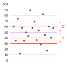
3. Standard Deviation: Provides a numerically meaningful measure of variance which represents the average distance each observation is from the mean.