Gaussian Distribution

Normal Distribution

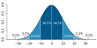
Normal (Gaussian) distribution is described as:

• a bell-shaped curve.
• valid for data that is symmetrically distributed around the mean.
• Parameter μ is the mean (location of the peak) and σ² is the variance (the measure of the width of the distribution).
• The distribution with μ = 0 and σ² = 1 is called the standard normal and the mean = median = mode

When a random variable X is distributed normally with mean μ and variance σ², we denote the normal distribution as:

Dark blue is less than one standard deviation from the mean. For the normal distribution, this accounts for about 68% of the set, while two standard deviations from the mean (medium and dark blue) account for about 95%, and three standard deviations (light, medium, and dark blue) account for about 99.7%.

• 68.2% of all scores cluster around the mean within approximately 1 standard deviation
• 95.4% within approximately 2 standard deviations
• 99.7% within approximately 3 standard deviations

Several biological variables are normally distributed (e.g., blood pressure, serum cholesterol, height, and weight). The normal curve can be used to estimate probabilities (frequency of occurrence) associated with these variables.

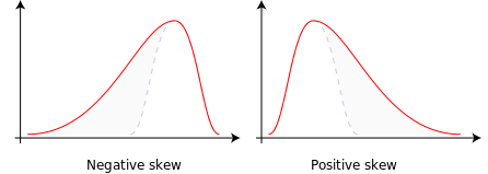
In real life, normal distributions are by far standard (μ ≠ 0, σ² ≠1) and tend to be skewed in the positive or negative direction:

• Negatively skewed: Example of values: 1,1000,1001,1002,1003. The tail is on the left, and there are relatively few low values and many high values. Median < Mean < Mode
• Positively skewed: Example of values: 1,2,3,4,100. The tail is on the right and there are relatively few high values and many low values. Mean > Median > Mode

A simple bimodal distribution, in this case a mixture of two normal distributions with the same variance but different means

The mode is least affected by the outliers of the sample. Some distributions show "disruption", rendering them bimodal (they have 2 humps). This shows that in the sampled population exist two distinct "sub-populations", that each one of them have their own normal distribution.

Confidence Interval (CI)

Confidence interval (CI): Used when, instead of simply wanting the mean value of a sample, we want a range that is likely to contain the true population value. The confidence interval denotes with a certain confidence (95%, 97%, etc) that the true value of the population mean within that interval. The narrower the CI, the more accurate the true (population) mean prediction is, but with a lower confidence. The opposite applies for a wide CI. The best combination is to have as large sample as possible with a non-wide CI (<99%).

When taking a sample for a normally distributed variable such as blood pressure, one sample of x people and another sample of x other people might have different means. This, of course, does not allow us to know the true value of the mean. The CI will denote a range of values in which both of these means will lie (if the samples were representative, non-biased and not small), but also the true population sample (which can be calculated if we measure the blood pressure of every human being).

Links

Bibliography

• HARRIS, Michael – TAYLOR, Gordon. Medical and Health Science Statistics Made Easy [online] . 2nd edition. Jones and Bartlett Publishers, 2009. Available from <http://books.google.com/books?id=WqVbhD69WvMC&lpg=PA16&ots=3KRluMt2GJ&dq=%22indicates%20how%20much%20a%20set%20of%20values%20is%20spread%20around%20the%20average.%22&hl=cs&pg=PP1#v=onepage&q=%22indicates%20how%20much%20a%20set%20of%20values%20is%20spread%20around%20the%20average.%22&f=false>. ISBN 9780763772659.

• BENCKO CHARLES UNIVERSITY, PRAGUE 2004, 270 P, V, et al. Hygiene and epidemiology. Selected Chapters. 2nd edition. Prague. 2008. ISBN 9788024607931.

Further reading

• Normal Distribution